STR module details
업데이트:
What Is Wrong With Scene Text Recognition Model Comparisons? Dataset and Model Analysis에서 등장하는 modele을 정리한 글입니다.
1. Transformation Stage
[STN] Spatial Transformer Network
[RARE] Robust Scene Text Recognition with Automatic Rectification
STN (Spatial Transformer Network)
- CNN max pooling : feature map을 축소하여, 분류 작업에 유리한 invariance를 얻을 수 있음. 예를 들어, 얼굴 인식에서 위치와 상관없이 눈, 코, 입을 인식할 수 있도록 한다.
- BUT! translation(위치)와 관계없이 동일하게 인식하지만, orientation(방향), proportion(비율) 등 달라지면 인식을 못한다. (물체를 바라보는 시점도 취약)
- data augmentation(다양한 방식으로 변형하여 이미지 생성)을 사용하면 이를 극복할 수 있으나 학습 시간이 길어진다.
- 이러한 CNN의 spatially inavariant(불변성)를 한계라고 생각하여 STN 등장하였다. (max pooling의 2*2 단위 연산으로는 data의 다양한 spatial vaiability(scale, rotation, translation) 대처하기 힘들다.)
-
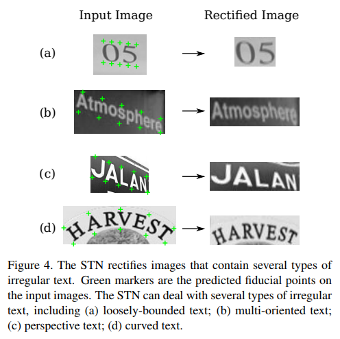
STN은 image 또는 feature map에서 관련 영역만 선택하여 가장 일반적인 형태로 변환 등 활용이 가능하다. 또한 scaling, cropping, rotation, non-grid deformation(thin plate spline) 등 지원한다.
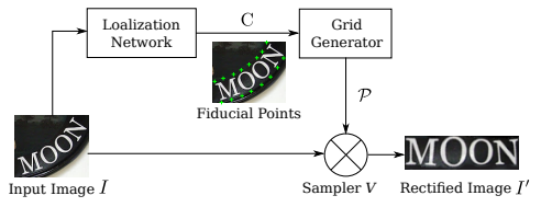
1.1 TPS transformation
- input image \(X\) -> normalized image \(\tilde X\)
- fiducial points set(F 개) 사이에서 smooth spline interpolation을 사용한다.
1) localization network
: finding a text boundary
- input image \(X\) 위에 존재하는 fiducial points의 x-y좌표 \(C\)를 계산한다.
- \(\tilde C\)는 초기화되는 좌표로, normalized image(rectified image)에서의 fiducial points를 의미한다.
\(C = [c_1, ... , c_F] \in \mathbb{R^{2*F}}, c_f = [x_f, y_f]^T\)
\(\tilde C\) : normalized image \(\tilde X\)의 pre-defined top & bottom location
RARE
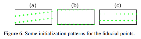
- 입력 이미지의 전체적인 텍스트 모양을 캡쳐하여, regressing을 통해 fiducial points F개의 위치를 찾아낸다. (fiducial points 개수는 짝수로, 여기서 20으로 초기화함)
\(C = [c_1, ... , c_F] \in \mathbb{R^{2*F}}, c_f = [x_f, y_f]^T\) - RARE[25]에서는 좌표는 [-1, 1] 범위안에 드는 normalized 좌표이다.
- regression을 위해 CNN을 사용한다. (classification이 아닌 regression을 위해 사용!!)
- RARE[25]에서는 [-1, 1] 범위 안에 있는 normalized 좌표로 C를 나타내고자 한다. 따라서, output layer(fully-connected layer)에서 output node를 2F로 하고, activation function으로 tanh을 사용하여 이러한 C를 만족하는 output vector를 가지도록 한다. 하지만, 이 논문에서는 activation function으로 ReLU를 사용하였다.
- fiducial points 좌표에 대한 샘플은 없다. 즉, localization network의 training은 back-propagation에 따라 STN의 다른 부분에 의해 전파된 gradients에 의해 supervise 된다. (ground truth 없이 오직 back propagation에 의해 조정한다)
2) grid generator
: linking the location of the pixels in the boundary to those of the normalized image
localization network에서 찾은 identified region과 normalized image(rectified image)를 연결하는 T를 찾는다.
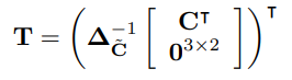 \(T \in \mathbb{R^{2*F+3}}\)
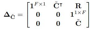 \(R = \{d_{ij}^2\}, d_{ij} =\)euclidean distance between \(\tilde c_i\) & \(\tilde c_j\)
3) image sampler
: generating a normalized image by using the values of pixels and the linking information
grid generator으로 결정된 input image의 픽셀을 interpolate하여 normalized image를 생성한다. 최종 output이 생성된다.
1.2 TPS-Implementation
TPS는 input image의 fiducial points를 계산하는 localization network를 필요로 한다. RARE[25]에서 사용한 요소에다가 Batch Normalization layers(BN)와 network의 training을 안정시키기 위해 adaptive average pooling(APool)을 추가한다.
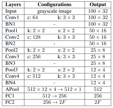
- 4 convolution layer + batch normalization layer + 2x2 max-pooling layer(마지막은 adaptive average pooling)
- 모든 convolution layer는 filter size = 3, padding size = 1, stride size = 1
- APool 이후, two fully connected layers : 512 to 256, 256 to 2F
- final output : 2F dimesional vector (input image의 F fiducial points x-y 좌표와 일치)
- 모든 layer의 activation function = ReLU
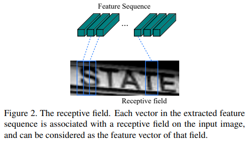
2. Feature Extration Stage
input image \(X\) or \(\tilde X\) -> feature map \(V = \{v_i\}, ( i = 1, ... , I )\) (num of columns in feature map)
- input channel = 1
- output channel = 512
2.1 VGG
[CRNN] An End-to-End Trainable Neural Network for Image-based Sequence Recognition and Its Application to Scene Text Recognition
* BN : Batch Normalization Layer
- CRNN[24], RARE[25]에서 사용한 VGG를 구현하였다.
CRNN
- CNN model로부터 convolution layer와 max pooling layer 가져온다. (fully-connected layer는 제거)
- 모든 image(input)는 같은 높이를 가지도록 조정한다.
- feature maps로부터 sequance of feature vectors(다음 단계 input)을 추출한다.
- vector는 feature map에서 column 기준 왼쪽에서 오른쪽 방향으로 생성된다.
- i번째 feature vector = 모든 feature map의 i번째 column (column의 넓이는 single pixel로 고정)
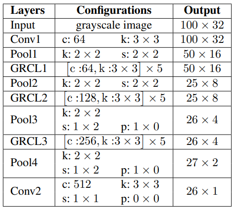
2.2 RCNN (recurrently applied CNN)
[GRCNN] Gated Recurrent Convolution Neural Network for OCR
-
gating mechanism으로 recursive하게 적용할 수 있는 RCNN인 Gated RCNN(GRCNN)을 구현하였다.
-
classification(물체 하나하나 인식)뿐만 아니라 object detection(bounding box로 다양한 object 인식)에서도 높은 성능을 보인다.
2.3 ResNet (Residual Network)
[ResNet] Deep Residual Learning for Image Recognition
-
FAN[4]에서 사용한 것과 동일한 network를 사용하였다.
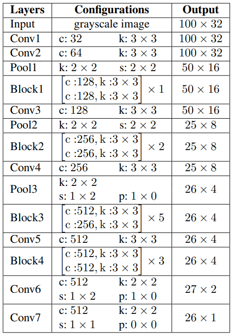
- neural network의 구조가 deep 할수록 vanishing/exploding gradient 문제로 정확도가 줄어든다. (weight 분포가 균등하지 않고 역전파가 제대로 이뤄지지 않기 때문이다.) ResNet은 이러한 문제를 해결하기 위해 제안되었다.
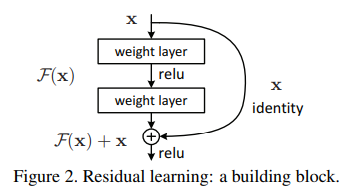
- residual learning
- 기존 네트워크 \(H(x)\)에서 \(F(x) = H(x) - x\)로 변형시켜 \(F(x) + x\)를학습시키는 것을 말한다.
- shortcut connection : \(y = \mathcal{F}(x, \{W_i\} + x)\)
- ResNet은 deep하더라도 더 좋은 성능을 보였다.
3. Sequence Modeling Stage
\[H = Seq.(V)\]3.1 BiLSTM (Bidirectional LSTM)
- CRNN[24]에서 사용한 2-layers BiLSTM을 구현하였다.
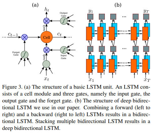
- FC layer를 포함한 모든 hidden state의 dimension은 256이다.
- Sequence module을 사용하지 않는 경우, H = V
recurrent layers를 사용할 때 장점
- RNN은 sequence 내에서 문맥 정보를 캡처하는 강력한 기능을 가진다.
- 문맥 정보를 이용하는 것이 독립적으로 처리하는 것보다 안정적이고 도움이 된다.
- 모호한 문자들은 문맥을 분석하면 더 구별하기 쉽다.
- ex) i , l : 개별적으로 인식하는 것보다 문자 높이를 비교하여 인식하는 것이 더 쉽다.
- CNN과 RNN을 공동으로 학습할 수 있다.
- RNN은
LSTM (Long Short Term Memory)
RNN(Recurrent Neural Networks)의 vanishing gradient problem을 극복하기 위해서 고안되었다. RNN의 hidden state에 cell state를 추가한 구조를 보인다.
(참고 : http://colah.github.io/posts/2015-08-Understanding-LSTMs/)
4. Prediction Stage
input \(H\) -> final prediction \(Y = y_1,y_2,...\) (sequence of characters)
C : character label set (37)
| pred. | examples |
|---|---|
| CTC | CRNN, GRCNN, Rosetta, STAR-Net |
| Attn | R2AM, RARE |
4.1 CTC (Connetionist Temporal Classification)
[CTC] An Intuitive Explanation of Connectionist Temporal Classification
- 음성 인식, OCR에서 많이 사용한다.
- character labe set C : 36 alphanumeric characters + 1 blank
1. Encoding
CTC Loss Function을 사용하기 위해 training 시작할 때 encoding을 하여 text sequence로 변환한다.
특별한 문자 blank를 사용하여 중복 문자 문제를 해결한다. 예를 들어 to와 too라는 단어를 encoding하면 다음과 같다.
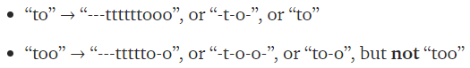
too를 too로 encoding하면, 이후 decoding할 때 to라는 단어로 예측할 수 있다. 이러한 중복 문제를 해결하기 위해 blank를 사용한다. 여기서 ‘-t-o’와 ‘to’, 그외에도 ‘too’, ‘t-oo’ 등은 모두 ‘to’를 가리키지만 이미지에서는 서로 다른 정렬을 보인다.
2. Decoding
best path decoding은 다음과 같다.
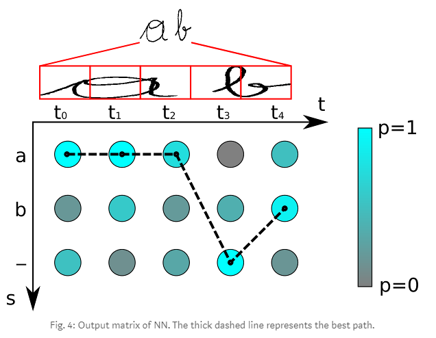
- 매 time step마다 가장 높은 확률을 가지는 문자를 선택한다. (aaa-b)
- 중복되는 문자를 먼저 제거하고, (a-b)
- 모든 blank를 제거한다. (ab)
3. Loss Function
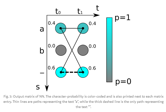
t는 time step이고, 세 가지 문자 {a, b, -}가 존재한다. 위의 그림을 따라 모든 경우에 대해 구할 수 있는데, 예를 들어 ‘aa’는 0.4*0.4 = 0.16이 나온다. 만약 ground truth 문자가 ‘a’라면, ‘aa’, ‘a-‘, ‘-a’에 대해 모두 합하여 0.64라는 것을 알 수 있다. 여기서 0.64는 loss가 아니라 ground truth의 probability를 의미하므로, loss는 probability의 음의 로그를 취하면 된다.
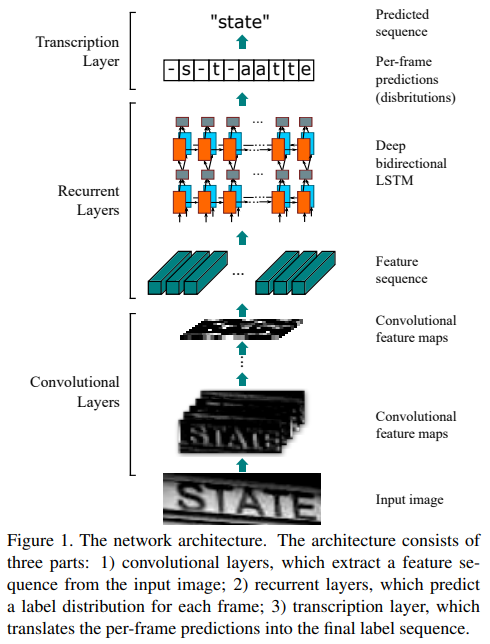
CRNN 구조 : None-VGG-BiLSTM-CTC
[CRNN] An End-to-End Trainable Neural Network for Image-based Sequence Recognition and Its Application to Scene Text Recognition
- 중복되는 문자를 제거한다. (-s-t-ate)
- blank(-)를 제거한다. (state)
4.2 Attn (Attention mechanism)
[FAN] Focusing attention: Towards accurate text recognition in natural images
[RARE] Robust Scene Text Recognition with Automatic Rectification
- FAN[4], AON[5], EP[2]에서 사용한 one layer LSTM attention decoder를 구현하였다.
- C : 36 alphanumeric characters + 1 EOS(end of sentence)
decoder는 \(y_t\)를 예측한다.
\[each\ step\ t, y_t = softmax(W_{_0S_t} + b_0)\]- \(W_0, b_0\) : trainable parameters
- \(s_t = LSTM(y_{t-1}, c_t, s_{t-1})\) : decoder LSTM hidden state at time t
- \(c_t\) : context vector = glimpse vector([FAN] AN은 glimpse vector를 생성시키고 FN은 reasonable한지 판단함)
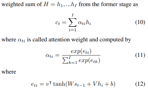
- \(\alpha_t\) : attention weight = alignment factors : input image의 attention region과 대응됨